Exploiting NDVI data from aerial image with Fiji (ImageJ)

Perhaps after all the work of making and calibrating your multicopter, you prepare your modified NIR camera, test the filters, stitch all the images together and get the final NDVI image through the PhotoMonitoring plugin and you may feel a bit dissapointed with the result. It was a hard work, the picture is beautiful, nice colors, etc.. but I feel there is something there but I couldn't tell what. At least this was my case, but it was before discovering the wonderful power of ImageJ. So I encourage you to go one step forward and exploit a little more that NDVI image so you can talk a bit more about it.

The features you may need depend on what is your photo about, but probably you may need to count specific elements in your photo (number of trees), or you may need to distinguish one type of elements from others (crop vs weed) and get differenciated measurements for each type.

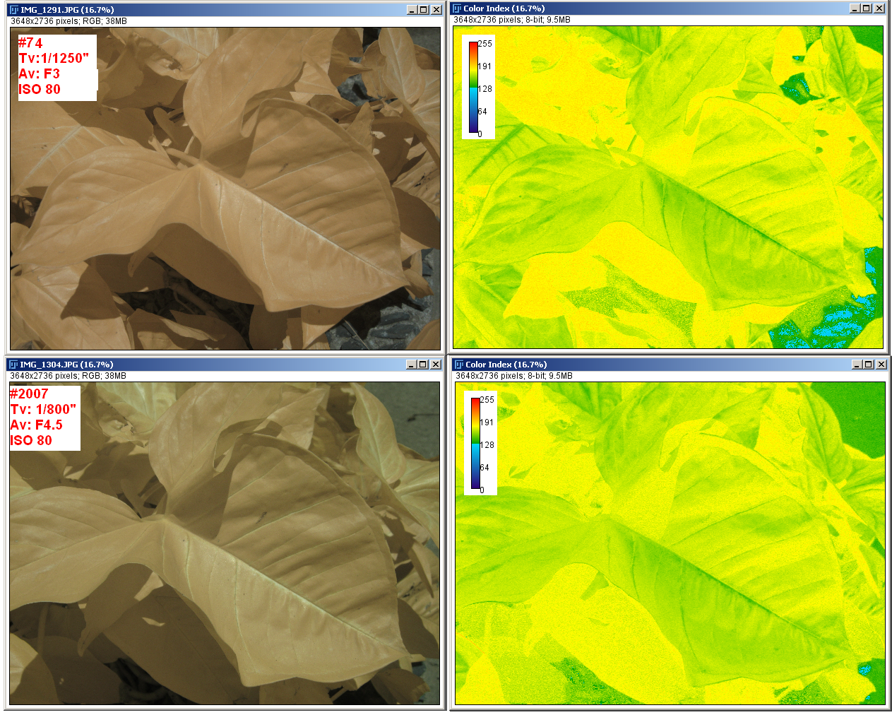
Here I present a simple sample of some of the feautures for a olive grove photo. This is the original NIR photo and the simple direct NDVI obtained with PhotoMonitoring Plugin of Fiji.

It is not easy to get much information from this NDVI image, the plugin maps from NDVI values ranging -1 to 1 to 0-255 and that values to color using the LUT. Healthy plants have NDVI values between 0.3 and 0.7, so we could limit the NDVI values to that range and map that range to 8bit color image, that way with the same color range (LUT) we could distinguish better the differences between the plants appearing in the photo. That is the most I expect to do, as I cannot trust the NDVI absolute values of this camera.

The floating point image containing NDVI information is a 32 bit depth grey scale image which we can easily threshold in Fiji to distinguish photosynthetic elements from the rest. The threshold feature classify gray scale images (there is also a color threshold) so values inside the threshold range are in in one group and the values outside it are in other group, so you can obtain statistics and use other features based on this classification.

32bit gray scale NDVI image [-1,1]

When applying the threshold (Image->Adjust-> Threshold) you are going to see the histogram of the image and two sliders for the bottom and top limits of the threshold (remember these are ndvi values as calculated by the plugin). I select just the zone of interest so I am sure that the values I am using for threshold correspond to the plants I want to study. There are several algorithms to be used but for now the default one is good. Mark "Dark background" if the elements of interest are brighter than the background, as in this case and choose the output colors for the thresholded image (B&W in this case). 

Threshold window

I think it is good to inspect the image with the mouse to have an idea of the values you are working with, I saw that in this image the trees never had values less than 0.1, so that gave me an idea of the lower limit for the threshold, with that in mind you can move the low limit slider until you see that just the trees an plants are visible, the top limit I leave it in 1.

NDVI thresholded image to [0.1,1]

Once the image is thresholded you will see a window with the results, that contains the information you are looking for, the lower and top limits of the NDVI values in the plants [0.106, 0.460], so I will use that range in the plugin to get a more easily interpretable color range in my result image:

Photomonitoring plugin values

I don't stretch the bands as all the information I have is meaninful and I don't want to remove any pixel. 

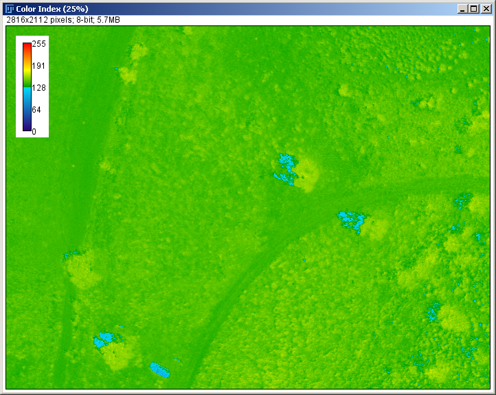
This is the new result, where it is more easily interpretable some zones in the grove where the ndvi values are higher than in others (more yellow and red colors)

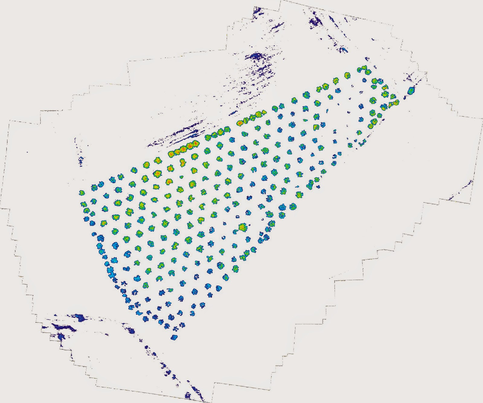
Color index image

Olive grove aerial DVI image

Mosaic composed of 184 photographs taken at 100m with a modified NIR camera (Canon A490 ) using a red filter.

DVI image obtained with Photo Monitoring plugin:

NDVI with red filters

Here a basic analysis about red filters performance for getting NDVI images. I compared four red filters:

The spectral response is similar, but it is sharper with #106, #19 and #135, and between these three, #19 and #135 have higher values and are supposed to be more luminous and easier for using fast shutter speed at as needed for aerial platforms. 

Here some photos with the three finalist filters:

#19 red fire

#135 golden amber

#106 primary red

To the naked eye the #135 appears with a brighter blue color, promising.


The NDVI images for each photo are the following (the visible channel used is Red and the NIR channel is Blue.)

#19

#135

#106

The #19 and #135 ndvi images are very similar and quite difficult to distinguish, but in the #106 there are lighter yellow colors and less presence of red is noticeable.

zoom comparative

Trying to get a more numerical value to base my decission I got the white balance coefficients used for each of the photos. With UfRaw for example you can get which were the camera coefficients used for the photo on each channel. The relation between Red and Blue channel coefficients could be used as an indicator of the goodness of the ndvi relative values. Doing that for each red filter and for each white balance used I got that the #135 golden amber gets the best relation with a custom white balance using a orange origami paper (and better with if it is white balanced in the shadow than in the direct sun light).

These NDVI values are not absolute of course, with just one camera and without knowing the sensor spectral response at NIR wavelenghts we just can get relative NDVI valuers, but using #135 filter and the proposed white balances a better interpretable NDVI photos can be achieved.

Comparing Rosco infrablue filters #2007 vs #74 for NDVI imaging

I am comparing here the results obtained with this two Rosco filters when getting NDVI images from NIR photos. The camera used was a Canon A490 with the IR filter previously removed. Camera was white balanced with a blue origami paper before taking photos with each filter. The software to process NIR photos was Fiji and Photomonitoring plugin.

The ideal criteria would be to compare NDVI values with real biological plant data, but as this is not possible for me I would compare photo histograms, that is objective data, and then interpret NDVI image, a more subjective analaysis.

Firstly it is interesting to compare filter spectral response. #74 lets less green wavelengths pass through and a bit less energy from blue channel, also less NIR wavelengths (> 700nm), so we can expect greater red-blue channel differences with #2007. The total area of passing wavelengths seems greater for #2007 so it will generate more luminous photos.

#74 filter above, #2007 below

This photo contains some plants and also some other objects that are not photosynthetic, I took this photo to evaluate filter ability to distinguish photosynthetic materia in an image.

The deduction about amount of light seems true as camera used faster shutter time for #2007. One curious thing is that leaf shadows appear with higher ndvi level than leafs, specially with #74. And also the shadow that crosses all the stone circle is noticeable in the #74 NDVI image, but not in the #2007. So one conclusion from this is that #74 is more affected by shadows and could lead to errors when distinguising plants in one image.

The histogram of each photo is the following. The difference between the average values of red and blue channel is 28,4 for #74 and 26,2 for #2007, what is not what I expected, but this full image histogram is not very meaningful as more than 75% of the photo is non photosynthetic material and the amount of plant reflecting more NIR is small. Anyhow I am comparing average values for each channel, which is a very rough analysis.

This other image is from just some leafs, all the objects in the image are photosynthetic so here we can evaluate better the ability of each filter to differentiate ndvi levels.

The histogram of the image reveals now a R-B everage difference of 62,1 with #74 and 56,2 for #2007. Here the comparison is for a image with 95% of photosynthetic material. And this small difference in channel levels is noticeable in the NDVI image, as the different levels in the main leaf are more clear in the #74 than in the #2007. 

The first conclusion is that #74 performs a bit better for my Canon A490 CCD, I will soon try the red filters as it is commented at Infragram that performs better than blue ones.

Getting good NDVI data from NIR infrablue aerial image

This aerial image was taken with a Canon A490 with the IR filter removed and with a piece of Rosco #2007 filter attached.

Exposure time: 1/1250"
F4.5
ISO 160

Focus: Single Point AF

Aerial image at 150m

I am testing this CHDK script for automatic exposure control, in the parameters you set a range of ISO, Av and Tv and the script calculates the best option at each photo. The only tricky issue with this script is that the lock focus and set focus to infinity doesn't work the same way on all cameras and if you are not lucky and the standard code doesn't work for you then you will have to figure out which are the right commands for your camera. I tested setting focus lock to infinity and also disabling lock focus and leaving the camera standard auto focus at each photo, and was getting better results with AF for my quad, camera, landscape configuration so I used that.

The purpose is to get a NDVI image and some insights on how proceed to get the best results given a set of amateur resources.

Rosco #2007 Infrablue filter

This infrablue filter is referred at Infragram to get better results with CCD cameras, although the results vary depending on the camera sensor (spectral response to NIR), camera settings (ISO, Av, Tv)  and white balance. I am using a custom white balance calibrated with a piece of blue origami paper, that is proven to get better results.

Rosco #2007 filter

Analyzing the color histogram of the photo can give us a hint of the quality of the resulting NDVI data. As NDVI is calculated from the difference of Red (NIR) and Blue channels, the separation between these two channels in the histogram is the key reference. For same scenario, the settings that get better separation os channels will likely get a more meaningful NDVI image. The main variables you can play with are:

- infrablue filter

- camera ISO, Av, Tv

- white balance

This is the color histogram of the entire image, that predicts a relatively good ndvi data as red and blue channels are at least well differenciated.

Color histogram from full image

This is the color histogram of just one tree (marked at the image with a yellow square), where the difference between the blue and red levels is more noticeable:

Tree selected for color histogram

Color histogram from one tree

NDVI images

This are the NDVI images obtained using Fiji and PhotoMonitoring plugin, the color difference between them is the lut used to map NDVI float values to color.

NDVI using NDVIBlu2Red lut from photomonitoring plugin

NDVI with special lut

Conclusions

1. Using a filter means that less light is reaching the sensor, and  that it will need longer exposure time to get the same energy, so Av and ISO should take this into account to get the shortest shutter speed and a clear photo. To get the same amount of light in less time lower F and higher ISO will help, but maintaining a reasonable range to avoid problems with too low F(too large deep of field, normally in aerial image we want the focus just in the ground) of too high ISO (noise). This image can help to understand:

This CHDK script can help you to get the best values for your specific situation: camera, ilumination, landscape colors, filter and uav performance about vibrations, but at the time of getting photos for a mosaic these values should be static, specially for getting a good NDVI mosaic where ndvi values can be compared between points that comes from different photos.

2. From the settings that influence the quality of the NDVI image, the only one that can be modified a posteriori is the white balance, and that just when you get a raw photo, so shooting raw will let us achieve better results. The downside of this is that taking the raw means more time between photo and photo, and that will impose a limit in your photo interval and then in the flight plan.

3. You can play with the lut to get the best  result according to the ndvi image purpose, from the above ones you can see that with the special one a best differentiation of live/dead object is seen.

4. Each camera will get better results with different filter, so you can take a know good combination of both or experiment by yourself.

5. White balance is critical to get good NDVI data, getting the best calibration of custom white balance is the key, and that depends on the light source at the momment of getting the photo, so this is something that should be done in situ before placing the camera in the uav.

CRIUS compass magnetic interference (compassmot)

The problem

I am using the CRIUS AIOP v2 flight controller, with MPNG 3.01 R3. I have been flying some months using auto modes without problems (loiter and auto missions). After a crash on a windy day I rebuilded the quad again using a H.A.L frame, as I am very pleased with the robustness and weight, and also price of it. This time I configured everything in the middle part to maintain the center of gravity as centered as possible, as my previous crash was produced messing around with different roll/pitch pid values trying to adapt to different weighted arms (camera and battery on one H.A.L arm).

With this new configuration, flying in auto missions some times at the time of changing from one waypoint to the next, in the momment of heading to face the next point the quad fails the angle and begin to fly in some random direction and I have to take manual control and bring it back home. This also happened in loiter, but just some times, it begins to lean one random angle and slowly fly away. I checked all the hardware parts without solving anything, in the end using compassmot I realized that I have a 65% of interference due to power cables, as this time the FC was about 1cm above the power cables, much closer than in any other configrations I did before.

Here a video of the effect at Loiter:

One solution

This was the original configuration, you can see the board  very close to the power cables (between thw two H.A.L. plater, near the orange plastic parts)

Hardware configuration with high magnetic interference

Detail of CRIUS FC position, 1cm above power cables

And the result of compassmot of 65%!!, using Attopilot current voltage and current sensor, properly configured in Mission Planner so in compassmot I was measuring current vs throttle:

65% Current vs Throttle interference

Here the new configuration, with the CRIUS FC 5cm above the power cables:

Hardware configuration with small magnetic interference

CRIUS FC board 5cm above power cables

The compassmot results shows a reduction to 10% interference, which results in a perfect loiter and auto mission performance. It is very important to do a new live compass calibration after moving the compass to other place, as offsets can vary significantly. I like also to do a live calibration periodically as recommended in the datasheet of the HMC5883L compass used in CRIUS, to take into account sensitivity drift due to temperature variations.

10% Current vs Throtle interference

If you cannot move away the FC then you can always use an external magnetometer I2C connected to the CRIUS board.

This is just one method to avoid magnetic interference, some others are described here, simple methods as twisting wires from battery to FC, and from FC to ESCs. For me this was the most effective as magnetic interference reduces with the cube of the distance to the source of the interference.

Magnetic interference

For a better understanding on how to solve one specific wiring ditribution on a quad it is good to understand a bit of the physics involved, simpliflying  the wire path from battery to flight board and then esc and return to battery as a circle (DC current, the one that produces most of the interference problem) :

The formula of magnetic field at a point at z axis, perpendicular to loop plane (Bz >> Bx, By, theoretically cancelled ina perfect loop), let us deduce some facts about how our wiring distribution would behave:

•  the bigger the circcle the stronger the magnetic field (proportional to R)
•  higher current implies higher interference (proportional to I)
•  the field reduces as the cube of the distance to the source (1/z3 proportional)
•  twisting the wires creates a sort of loop along the z plane (each twist one loop) that makes Bz somehow cancel itself along z axis, or at least been reduced.

Balancing multirotor motors with MMA8452Q accelerometer

This post is about using the MMA8452Q acceleromter to balance multirotor motors. As there is alot of information in the net about the balancing procedure I am focusing on using this cheap accelerometer for that purpose.

The easier way would be to use some app in a 3g phone to get and idea of the vibrations at the motor, but I lost my phone a month ago and I was living happy without it and didn't wat to spend 300$ in a new one. So searching for cheap and easy to set up accelerometers, this is one of them: less than 10$, I2C interface, 12bit resolution and example code.

MMA8452Q hw & sw setup

The connections is quite straigth forward, just solder some wires and connect to and arduino for example. This is form the example code MMA8452Q_AdvancedExample at GitHub

 Hardware setup:
 MMA8452 Breakout ------------ Arduino
 3.3V --------------------- 3.3V
 SDA ----------------------- A4
 SCL ----------------------- A5
 INT2 ---------------------- D3
 INT1 ---------------------- D2
 GND ---------------------- GND

It is possible to interface directly from a 3.3V device to a 5V arduino because SDA&SCl pull-ups at Arduino are disabled . For this you must use the i2c.h file in the example instead of the standard Wire arduino library, that switch on the pull-ups (twi.c):

void twi_init(void)
{
  // initialize state
  twi_state = TWI_READY;
  twi_sendStop = true; // default value
  twi_inRepStart = false;

  // activate internal pullups for twi.
  digitalWrite(SDA, 1);
  digitalWrite(SCL, 1);
  // initialize twi prescaler and bit rate
  cbi(TWSR, TWPS0);
  cbi(TWSR, TWPS1);
  TWBR = ((F_CPU / TWI_FREQ) - 16) / 2;
  /* twi bit rate formula from atmega128 manual pg 204
  SCL Frequency = CPU Clock Frequency / (16 + (2 * TWBR))
  note: TWBR should be 10 or higher for master mode
  It is 72 for a 16mhz Wiring board with 100kHz TWI */
  // enable twi module, acks, and twi interrupt
  TWCR = _BV(TWEN) | _BV(TWIE) | _BV(TWEA);
}

The reason why this works is well explained in a comment in the product page at sparkfun, it is due to the open drain design of the i2c data lines. From sparkfun they notice that even without disabling the arduino pull-ups it works, and some users confirm it, because the final high voltage at the sensor input sda and scl lines would be 3.79V as a combination of sparkfun board 10k pull-ups to 3.3v and arduino 25k pull-ups to 5v, but I prefer to stay in the datasheet ranges, so I  disabled pull-ups at arduino.

I don't know why, but even reading in the sensor datasheet that a 4.7 ohms resistor is recommended as pull-up, sparkfun soldered 10k pull-ups in the board. Some users advice that seing signal at oscilloscope it appears quite rounded with 10k, and that it is better shaped with 4.7k, you can solder a paralell 10k to get 5k final resistante to pull-up, but I must say it works quite fine for me with the 10k resistors in the board.

Changing scale +/- 2g/4g/8g

It is neccesary to understand the Zero-g offset concept to understand the output values from the sensor. When stationary the output registers from the sensor will be 0x00 (ideally middle of dynamic range) , but in fact z g is 1g when laying flat and stationary. It is well explained in the application note AN4069.

At each scale each count from the ouput register means a different value of g. For example when the full-scale is set to 2g, the measurement range is -2g to +1.999g, and each count corresponds to 1g/1024

(1 mg) at 12-bits resolution, each count will mean double g value if scale is doubled to 4g, and same for 8g.

Then the value of counts stored in the offset registers are referred to a scale, and the value added to 0x00  output when flat and stationary to get 1g at z axis will only result in 1g when the scale is the same at which the calibration was done.

This can be confusing using the example code, if you change the default scale to 4g, you will get at flat and stationary : x=0g,y=0g and z=2g, and  x=0g,y=0g and z=4g when scale is 8g. You need to recalibrate if you want to see a pretty 1g for z, or if not at least understand what that value means.

Regarding scale also take into account that the scale is limited to 4g if you use the low noise mode, that is actiuvated by default in the example code

Using accelerometer data to balance multirotor motor

The procedure to balance a motor is well documented online, the idea is to place a weigth on different parts of the motor and compare the vibrations on each point. I did it using a ziptie and moving the head of the ziptie around the perimeter of the motor. In an ideal motor the vibrations woould be the same on every point, but in an unbalanced motor the vibrations will be less in the point where it is lighter.

You can plot the data in a easy way using Processing for example, that is what I tried first, but it is quite difficult to distinguish the difference in vibration level between two points simply observing the graphic. So I found it better to calculate mean value over time and comparing that mean at each point. That is an advantage of using arduino instead of a graphical phone application. If you sum up the mean on each axis you can get an idea of the overall vibrations generated by the motor. That all-axis mean cannot be used to compare vibrations between different motors unless you place the sensor equally leveled on all the motors, as z axis g value depends on the sensor horizontal level. But that all-axis mean can be used to compare vibrations in one motor placing the weigth at different points:

Summarizing the method:

1. Place the sensor on one motor, measure mean gx,gy,gx (about 3000 samples) and calculate gx+gy+gz = overall_g
2. Note values for (a) Motor alone (b) Ziptie at 4 positions separated 90 degrees
3. Put some weigth ( tape for instance) on the position where overall_g was less using the ziptie
4. Measure overall_g with the motor with that weigth and compare to value of motor alone in point 2, it should be less than alone.
5. Add weigth on that point while the overall_g continues decreasing until it start to increase.

With this method I got between 0,2g and 0,6g less overall vibration placing tape at the motors. I did it with the motors attached to the multirotor and spinning one at a time.

CRIUS AIOP v2 - Altitude hold based on MS5611 barometer

Some notes about the barometer included in the CRIUS AIOP flight controller and the importance of covering it with dark foam. I read some times about foam covering and I interpreted it as a way of getting more precise measurements, I expected to have some variance (cms, or 1, 2 meters as much)  if  you didn't cover it, but in fact it is absolutely necessary for being able to trust altitude measurements. Altitude is used in almost all common flight modes but Stailize and Acro (Auto, Altitude Hold, RTL, Loiter... )

The barometer used in CRIUS AIOP v2 is the MS5611-01BA03. This is an update from the MS5611-01BA01 used in previous versions of CRIUS board, but apart from the change from ceramic to metal case and slightly better response to variations in supply voltage, the specifications are same.

Having a quick look at the datasheet you see that the pressure calculated value depends on temperature, as the sensitivity of the sensor varies with it. Indeed there is a different calculation method for pressure when the temperature is below 20 degrees. This should not worry much if you fly in a cold day as long as the tempreature at the sensor remains more or less constant, but it would worry me if the temperature at the sensor suffers a dramatic change, say from 20 to 15 degrees in a very short time (due to a fresh air flow from the props for instance). It could easily led you from an altitude value of 10m to 500m, with the corresponding reaction from the copter....This kind of issue is what you can suffer if the sensor is exposed to sunlight or propwash.

I learned it by the hard way, the first flight with the sensor completely exposed gave me altitude values that varied as much as 500m from one momment to the other, just imagine the reactions from the multicopter when I was on any auto mode. 

In this log it can be seen the variations of 500m while trying to do a RTL (throttle in blue represent the reactions to such an altitude change, red is altitude, green is desired altitude)

So I covered the sensor with foam and introduced all the electronics into a dark box. I tried before just covering the sensor, but the altitude values were jumpy sometimes due to sunligth, for example one day I suffered a crash when the weather changed from foggy to shiny while copter was in the air. Conclusion: both air flow from propwash and sunligth produce important variations in temperature at the sensor, and in measured pressure therefore, so keep it calm and dark.

after that changes the values from the sensor were quite precise and now I can enjoy of rock solid loiters and auto missions. Here an example of the last log, you can't even distinguish the line of the desired altitude behind the real altitude:

And here a video demonstration of the perfect Loiter performance:

Quadcopter data:

- CRIUS AIOP v2
- MPNG 3.0.1 R2 firmware
- NTM 800kv 300W motors
- Graupner 12x6 props
- Rctimer 30A ESC with Simonk.

Multicopter KK2.1 MPU6050 Settings

This post is about MPU6050 Gyro+Acceleromter settings on the Hobbyking KK2.1 Flight Controller board. The meaning of these settings didn't seem obvious to me, neither the effect on how to multicopter would fly with different values so I write this to help me and others to get a deeper understanding on it. These settings are available from the menu of the Steveis firmware version. Here you can get last version, mine is 1.11S1 (December 2013)

Full Scale Range

The values for Gyro(deg/sec) and Acc(+/-g) are the full scale range of each sensor. The MPU6050 can be configured with different scale ranges, individually for Gyroscopes and Accelerometers:

MPU6050 uses 16bit sigma-delta ADC for gyros and accs. Examining the values in the above tables we can know the minimun value that can be measured with each scale range, that is defined by the value of 1 bit (LSB) in sensor units.

So the conclusion of this is that for a bigger range we get a less accurate measurement, as the minimum value (Least Significant Bit) increases. For example, with a range of +-16g for the accelerometer we just can distinguish values of 0.49mg, while it is 0.06mg for a scale of +-2g.

For getting advantage of this knowledge we should know what are the values that occurs in a multicopter in the air, values produced by wind or by user input. Then we should set the minimum necessary range to cover our work values, so we have the best possible accuracy and also because of what is mentioned below.

I couldn't get any schematic of the internals of MPU6050, but I suppose that roughly it is something like this (taken from the Analog Devices AN-396 accelerometer),

Basically a pre amplifier followed by an amplifier which gain is what is modified to change the scale factor. So, as it is recommended in its datasheet, never use more gain than is needed to provide a convenient scale factor, as the buffer gain not only amplifies the signal but any noise or drift as well. So the ideal range will be the minor one while covering the range of deg/sec and g the multicopter will move.

I don't know yet acceleration values (g) or angles rate of change (deg/sec) that a multicopter is exposed. I depends of course on the type of flying you are doing (acro or smooth fpv).  I plan to take them from experimental values using the logging function on my CRIUS AIOP 2.0. One reference I have found is this from a technical article on context recognition, that could give an idea of acceleration of well known movements for us:

Low pass Filter

The MPU6050 has a user programmable low pass filter that affects equally to gyro and accelerometer. These are the possible frequency values:

  

In the end this value is used to filter unwanted deviations due to noise or vibrations affecting the multicopter, beacuse meaningful changes due to user input or wind are not supposed to have a frequency greater than 250Hz (1/250Hz = 4ms).

Just to help a little bit more, I leave this comment from the multiwii MPU6050_config.h config file, it is not a KK2.1 software but the information could be useful to understand the effects of LPF on multicopter behaviour:

/* MPU6050 Low pass filter setting. In case you cannot eliminate all vibrations to the Gyro, you can try
   to decrease the LPF frequency, only one step per try. As soon as twitching gone, stick with that setting.
   It will not help on feedback wobbles, so change only when copter is randomly twiching and all dampening    and balancing options ran out. Uncomment only one option!
   IMPORTANT! Change low pass filter setting changes PID behaviour, so retune your PID's after changing LPF.*/